Universal Approximation: A Finite-Dimensional Approach

This note presents constructive approximation theorems for both polynomials and neural networks using primarily finite-dimensional linear algebra. We rely on the tools from our analysis review (vector norms, inner products, Cauchy-Schwarz, matrix norms) plus standard calculus results (Taylor's theorem, continuous function properties).

Main Result (Universal Approximation): Let $f: [a,b] \to \mathbb{R}$ be any continuous function, and let $\epsilon > 0$ be an error tolerance. We will prove that:

Polynomials: There exists a polynomial $p(x)$ such that $$\max_{x \in [a,b]} |f(x) - p(x)| < \epsilon$$
Neural Networks: There exists a one-hidden-layer ReLU network $f_{NN}(x)$ such that $$\max_{x \in [a,b]} |f(x) - f_{NN}(x)| < \epsilon$$

Both approximators use $O(\epsilon^{-c})$ parameters for some constant $c$. The proofs are constructive - we explicitly build the approximators and bound their errors.

1. Function Approximation on Finite Grids

1.1 Setup: Discretizing the Problem

Proposition (Norm Equivalence): For any $\mathbf{f} \in \mathbb{R}^{N+1}$: $$\|\mathbf{f}\|_\infty \leq \|\mathbf{f}\|_2 \leq \sqrt{N+1} \|\mathbf{f}\|_\infty$$

Proof: The first inequality follows from the definition. For the second: $$\|\mathbf{f}\|_2^2 = \sum_{i=0}^N f_i^2 \leq \sum_{i=0}^N \|\mathbf{f}\|_\infty^2 = (N+1) \|\mathbf{f}\|_\infty^2$$ Taking square roots gives the result. □

1.2 Error Measurement

2. Polynomial Approximation

2.1 Lagrange Interpolation

Theorem (Existence of Interpolating Polynomial): Given $n$ distinct points $(x_0, y_0), \ldots, (x_{n-1}, y_{n-1})$ with $x_i \in [a,b]$, there exists a unique polynomial $p(x)$ of degree at most $n-1$ such that: $$p(x_i) = y_i, \quad i = 0, 1, \ldots, n-1$$

Proof:

Step 1 (Linear System): Write $p(x) = c_0 + c_1 x + \cdots + c_{n-1} x^{n-1}$. The interpolation conditions give: $$\begin{bmatrix} 1 & x_0 & x_0^2 & \cdots & x_0^{n-1} \\ 1 & x_1 & x_1^2 & \cdots & x_1^{n-1} \\ \vdots & \vdots & \vdots & \ddots & \vdots \\ 1 & x_{n-1} & x_{n-1}^2 & \cdots & x_{n-1}^{n-1} \end{bmatrix} \begin{bmatrix} c_0 \\ c_1 \\ \vdots \\ c_{n-1} \end{bmatrix} = \begin{bmatrix} y_0 \\ y_1 \\ \vdots \\ y_{n-1} \end{bmatrix}$$

Step 2 (Vandermonde Determinant): The matrix $V$ is the Vandermonde matrix. A standard result from linear algebra states: $$\det(V) = \prod_{0 \leq i < j \leq n-1} (x_j - x_i)$$ Since all $x_i$ are distinct, each factor $(x_j - x_i) \neq 0$, so $\det(V) \neq 0$ and $V$ is invertible.

Since $\det(V)$ has degree $n-1$ in $x_{n-1}$ and has $n-1$ roots, we can write: $$\det(V) = C \prod_{i=0}^{n-2} (x_{n-1} - x_i)$$ for some constant $C$ (which may depend on $x_0, \ldots, x_{n-2}$).

To find $C$, look at the coefficient of $x_{n-1}^{n-1}$ in $\det(V)$. By cofactor expansion along the last row, this coefficient comes from the $(n-1) \times (n-1)$ Vandermonde minor obtained by deleting the last row and column, which by induction has determinant: $$C = \prod_{0 \leq i < j \leq n-2} (x_j - x_i)$$

Combining gives the full formula. □

Since all $x_i$ are distinct, $\det(V) \neq 0$, so $V$ is invertible.

Combining gives the full formula. □

Since all $x_i$ are distinct, $\det(V) \neq 0$, so $V$ is invertible.

Step 3 (Unique Solution): The coefficient vector is $\mathbf{c} = V^{-1} \mathbf{y}$, which is unique. □

Corollary (Zero Error on Grid): The interpolating polynomial achieves: $$\|\mathbf{p} - \mathbf{f}\|_2 = \|\mathbf{p} - \mathbf{f}\|_\infty = 0$$ on the discrete grid points.

2.2 Explicit Construction: Lagrange Basis

Theorem (Lagrange Interpolation Formula): $$p(x) = \sum_{j=0}^{n-1} y_j L_j(x)$$

Proof: Direct verification: $$p(x_i) = \sum_{j=0}^{n-1} y_j L_j(x_i) = \sum_{j=0}^{n-1} y_j \delta_{ij} = y_i$$ The polynomial has degree at most $n-1$ and satisfies all interpolation conditions, so by uniqueness, this is the interpolating polynomial. □

2.3 Convergence on Uniform Grids via Partition of Unity

Using the partition of unity property, we can prove that Lagrange interpolation on uniform grids converges to smooth functions as the grid is refined.

Theorem (Interpolation Error on Uniform Grids): For a smooth function $f$ and Lagrange interpolant $p(x)$ using $n+1$ uniform nodes with spacing $h$: $$|f(x) - p(x)| = O(h^{n+1})$$ as $h \to 0$, provided $f$ has $n+1$ continuous derivatives.

Proof idea: Start with the Taylor expansion of $f(x_j)$ about any point $x$: $$f(x_j) = f(x) + f'(x)(x_j - x) + \frac{f''(x)}{2}(x_j - x)^2 + \cdots + \frac{f^{(n+1)}(\xi_j)}{(n+1)!}(x_j - x)^{n+1}$$ The Lagrange interpolant is: $$p(x) = \sum_{j=0}^{n} f(x_j) \ell_j(x)$$ Substituting the Taylor expansion: $$p(x) = \sum_{j=0}^{n} \left[f(x) + f'(x)(x_j - x) + \cdots \right] \ell_j(x)$$ Distribute the sum: $$p(x) = f(x) \underbrace{\sum_{j=0}^{n} \ell_j(x)}_{=1} + f'(x) \underbrace{\sum_{j=0}^{n} (x_j - x)\ell_j(x)}_{=0} + \cdots$$ Key observation: By the partition of unity property, the first sum equals 1. The higher-order sums vanish because Lagrange interpolation exactly reproduces polynomials of degree $\leq n$. Specifically, if we interpolate the polynomial $g(y) = (y-x)^k$ for $k \leq n$, we get back exactly that polynomial, so evaluating at $y=x$ gives zero: $$\sum_{j=0}^{n} (x_j - x)^k \ell_j(x) = 0, \quad k = 1, 2, \ldots, n$$ Therefore, all the polynomial terms in $p(x)$ match $f(x)$ exactly, leaving only the remainder: $$f(x) - p(x) = -\sum_{j=0}^{n} \frac{f^{(n+1)}(\xi_j)}{(n+1)!}(x_j - x)^{n+1} \ell_j(x)$$ For piecewise interpolation with fixed degree $n$, we divide the domain into small intervals, each of width $O(h)$. On each interval, we use $n+1$ nodes with spacing $h$, so $|x_j - x| \leq nh$. Since $n$ is fixed, $nh = O(h)$. Taking absolute values: $$|f(x) - p(x)| \leq \frac{\max |f^{(n+1)}|}{(n+1)!} h^{n+1} \sum_{j=0}^{n} n^{n+1} |\ell_j(x)|$$ The sum $\sum_j |\ell_j(x)|$ is bounded by a constant depending only on $n$. Therefore: $$|f(x) - p(x)| = O(h^{n+1})$$ Important caveat: This analysis assumes piecewise interpolation where $n$ is fixed and we refine by decreasing $h$. For global interpolation over a fixed domain $[a,b]$ with $n+1$ points, the interval width is $nh \approx b-a = O(1)$ (constant), not $O(h)$, and the basis functions grow exponentially with $n$ (Runge phenomenon). □

Concrete Examples (Piecewise Interpolation):

Piecewise linear ($n=1$): Divide domain into intervals of width $h$. On each interval, use 2 points. The maximum distance is $|x_j - x| \leq h$, and $\sum_j |\ell_j(x)| \leq 2$: $$|f(x) - p(x)| \leq \frac{h^2}{8} \max |f''(x)|$$

Piecewise quadratic ($n=2$): Divide domain into intervals of width $2h$. On each interval, use 3 points with spacing $h$. The maximum distance is $|x_j - x| \leq 2h$, giving: $$|f(x) - p(x)| = O(h^3)$$

Strategy for accuracy:

Piecewise approach: Fix $n$ (degree), refine mesh by decreasing $h$ → error decreases as $O(h^{n+1})$
Global approach: Fix domain size, increase $n$ → Runge phenomenon (error can grow!)

Finite element methods use the piecewise approach: low-degree polynomials on many small elements.

2.4 Polynomial Approximation (Not Interpolation)

The Lagrange interpolation approach forces exact agreement at grid points, which can lead to oscillations between points (the Runge phenomenon). However, if we allow small errors at grid points, polynomials can achieve excellent uniform approximation.

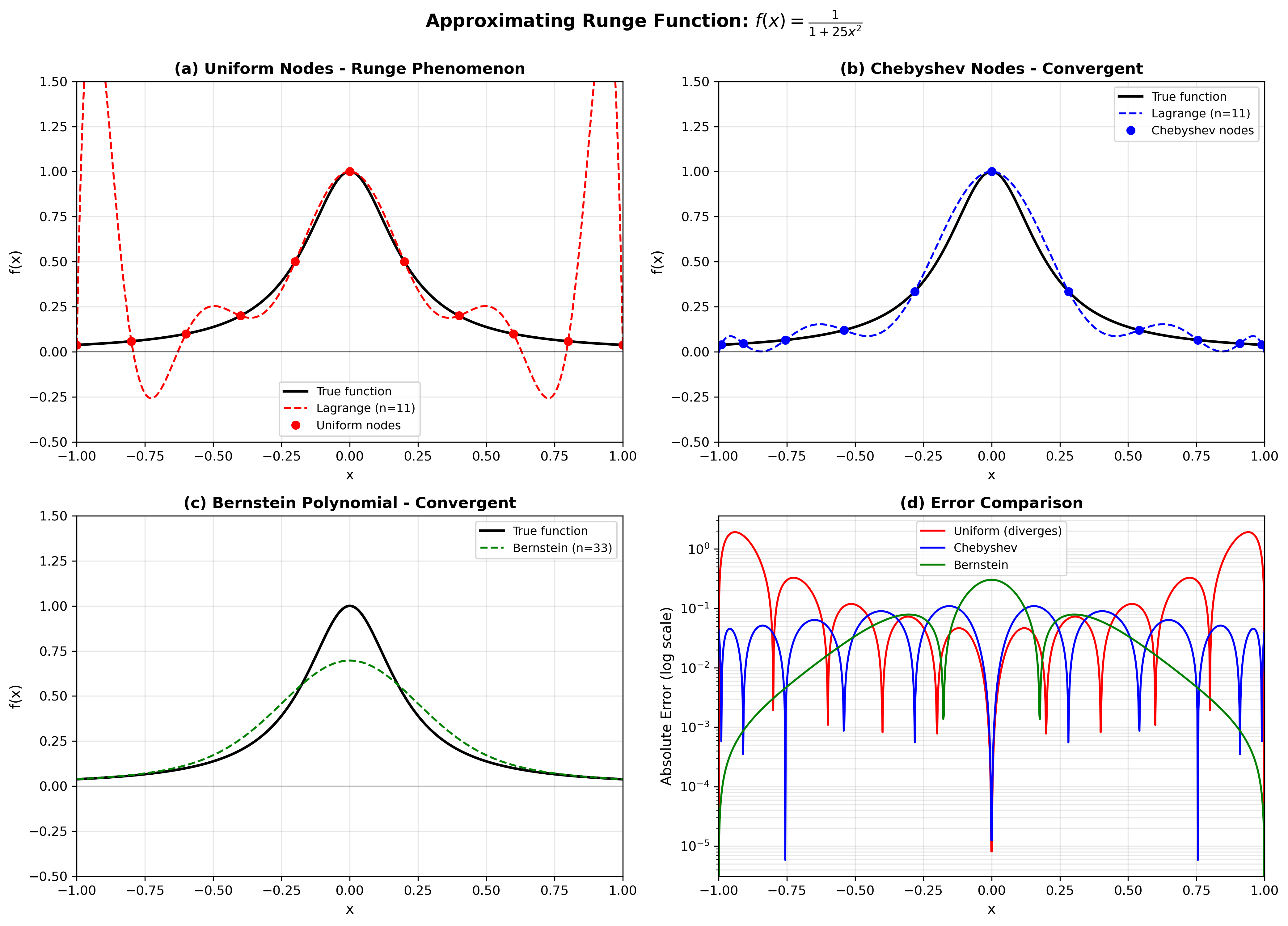
Figure 1: Comparison of approximation methods for the Runge function $f(x) = \frac{1}{1 + 25x^2}$ with $n=11$ nodes. (a) Lagrange interpolation on equally-spaced nodes exhibits large oscillations near the boundaries (Runge phenomenon). (b) Lagrange interpolation on Chebyshev nodes converges stably without oscillations. (c) Bernstein polynomials (degree 33) provide uniform convergence. (d) Error comparison on log scale demonstrates that uniform interpolation diverges while Chebyshev and Bernstein methods converge.

2.5 Uniform Polynomial Approximation with Error Control

Instead of requiring $p(x_i) = f_i$ exactly, we can construct polynomials that minimize the worst-case error over the entire interval.

Theorem (Constructive Polynomial Approximation): Let $f: [a,b] \to \mathbb{R}$ be continuous. For any $\epsilon > 0$, there exists a Bernstein polynomial $B_n(f)$ of degree $n = O(\epsilon^{-2})$ such that: $$\max_{x \in [a,b]} |f(x) - B_n(f; x)| < \epsilon$$ For smooth functions $f \in C^2[a,b]$ with $|f''(x)| \leq M$, the convergence rate is $O(n^{-1})$.

Proof idea (Bernstein Polynomials):

Construction: For $f$ on $[0,1]$, the $n$-th Bernstein polynomial is: $$B_n(f; x) = \sum_{k=0}^n f\left(\frac{k}{n}\right) \binom{n}{k} x^k (1-x)^{n-k}$$ The basis functions $b_{n,k}(x) = \binom{n}{k} x^k (1-x)^{n-k}$ form a partition of unity: $\sum_{k=0}^n b_{n,k}(x) = 1$.

Key property: The error can be written: $$|f(x) - B_n(f; x)| = \left|\sum_{k=0}^n \left[f(x) - f\left(\frac{k}{n}\right)\right] b_{n,k}(x)\right|$$ By uniform continuity, when $|k/n - x|$ is small, $|f(k/n) - f(x)|$ is small. The Bernstein basis has a "concentration" property: as $n \to \infty$, most of the weight $b_{n,k}(x)$ is concentrated near $k/n \approx x$. This can be quantified using the variance bound: $$\sum_{k=0}^n \left(\frac{k}{n} - x\right)^2 b_{n,k}(x) \leq \frac{1}{4n}$$ Combining uniform continuity with this concentration property proves that $B_n(f) \to f$ uniformly, with degree $n = O(\epsilon^{-2})$ for general continuous functions. For $C^2$ functions, the rate improves to $n = O(\epsilon^{-1})$. □

Takeaway: Polynomials can approximate any continuous function, but the tradeoff between degree and accuracy depends on the function's smoothness.

2.5 Alternative: Chebyshev Nodes for Interpolation

Another approach is to use non-uniform grid points that avoid Runge phenomenon.

Theorem (Chebyshev Interpolation Error): For $f \in C^k[-1,1]$, the Lagrange interpolation polynomial at Chebyshev nodes satisfies: $$\max_{x \in [-1,1]} |f(x) - p(x)| \leq \frac{2}{k!} \left(\frac{1}{n}\right)^k \|f^{(k)}\|_\infty$$

Key Insight: Unlike equally-spaced points, Chebyshev interpolation converges for smooth functions, with error $O(n^{-k})$ for $f \in C^k$.

2.6 Remark on the Runge Phenomenon

Important Clarification: The Runge phenomenon occurs for polynomial interpolation on equally-spaced points. It does NOT mean polynomials are inferior approximators! With proper choices:

Moral: Both polynomials and neural networks require careful construction. The choice of grid/nodes matters as much as the choice of basis functions!

3. Neural Network Approximation

3.1 One-Hidden-Layer Networks

3.2 Building Blocks: ReLU Functions

Proof of Hat Function Construction:

Step 1: Define the building blocks:

$\sigma(h(x - x_{i-1}))$ creates a ramp starting at $x_{i-1}$
$-2\sigma(h(x - x_i))$ creates a downward ramp starting at $x_i$
$\sigma(h(x - x_{i+1}))$ creates an upward ramp starting at $x_{i+1}$

Step 2: Verify at key points:

At $x = x_{i-1}$: $\phi_i = \frac{1}{h}[0 - 0 + 0] = 0$
At $x = x_i$: $\phi_i = \frac{1}{h}[h - 0 + 0] = 1$
At $x = x_{i+1}$: $\phi_i = \frac{1}{h}[2h - 2h + 0] = 0$

Step 3: Check linearity in each interval by differentiation: $$\phi_i'(x) = \begin{cases} 1/h & x \in (x_{i-1}, x_i) \\ -1/h & x \in (x_i, x_{i+1}) \\ 0 & \text{otherwise} \end{cases}$$ This gives the piecewise linear hat shape. □

3.3 Piecewise Linear Interpolation with Neural Networks

Theorem (Neural Network Interpolation): Given grid points $(x_0, f_0), \ldots, (x_N, f_N)$ on $[a,b]$, there exists a one-hidden-layer ReLU network with $O(N)$ neurons such that: $$f_{NN}(x_i) = f_i, \quad i = 0, 1, \ldots, N$$ and $f_{NN}$ is piecewise linear between grid points.

Proof (Construction):

Step 1 (Basis Expansion): Define: $$f_{NN}(x) = \sum_{i=0}^N f_i \phi_i(x)$$ where $\phi_i$ are the hat functions from the previous lemma.

Step 2 (Verification at Grid Points): By the Kronecker property $\phi_i(x_j) = \delta_{ij}$: $$f_{NN}(x_j) = \sum_{i=0}^N f_i \delta_{ij} = f_j$$

Step 3 (Neuron Count): Each interior hat function $\phi_i$ ($i = 1, \ldots, N-1$) requires 3 ReLU neurons. The boundary hat functions $\phi_0$ and $\phi_N$ each require 2 neurons. Total: $$3(N-1) + 2 \cdot 2 = 3N - 3 + 4 = 3N + 1 \text{ ReLU activations}$$ (Plus bias adjustments, giving approximately $3N$ neurons). □

Corollary (Zero Error on Grid): Like polynomial interpolation: $$\|\mathbf{f}_{NN} - \mathbf{f}\|_2 = \|\mathbf{f}_{NN} - \mathbf{f}\|_\infty = 0$$ on the discrete grid.

3.4 Between-Grid Behavior

Key Difference from Polynomials: The neural network approximation $f_{NN}$ is:

Proposition (Boundedness): For the constructed $f_{NN}$: $$\|f_{NN}\|_{C[a,b]} = \max_{x \in [a,b]} |f_{NN}(x)| \leq \|\mathbf{f}\|_\infty$$

Proof: Since $\sum_i \phi_i(x) = 1$ for all $x \in [a,b]$ (partition of unity): $$|f_{NN}(x)| = \left|\sum_i f_i \phi_i(x)\right| \leq \sum_i |f_i| \phi_i(x) \leq \|\mathbf{f}\|_\infty \sum_i \phi_i(x) = \|\mathbf{f}\|_\infty$$ by the triangle inequality and non-negativity of $\phi_i$. □

Remark: This boundedness property prevents Runge-like oscillations. The neural network cannot "explode" between grid points.

4. Comparison and Error Analysis

4.1 Approximation of Smooth Functions

Assumption: Suppose $f \in C^2[a,b]$ with $|f''(x)| \leq M$ for all $x \in [a,b]$.

Theorem (Piecewise Linear Approximation Error): For the neural network $f_{NN}$ constructed from grid values: $$\max_{x \in [a,b]} |f(x) - f_{NN}(x)| \leq \frac{M h^2}{8}$$ where $h = (b-a)/N$ is the grid spacing.

Proof:

Step 1 (Localization): It suffices to bound the error on each subinterval $[x_i, x_{i+1}]$.

Step 2 (Linear Interpolation on Subinterval): On $[x_i, x_{i+1}]$, the neural network is: $$f_{NN}(x) = f_i + \frac{f_{i+1} - f_i}{h}(x - x_i)$$

Step 3 (Standard Interpolation Error Formula): For a twice-differentiable function $f$ on $[x_i, x_{i+1}]$, a standard result from calculus/numerical analysis states that the error in linear interpolation is given by: $$f(x) - f_{NN}(x) = \frac{(x - x_i)(x - x_{i+1})}{2} f''(\xi)$$ for some $\xi \in (x_i, x_{i+1})$. This follows from Taylor's theorem applied to both endpoints.

Step 4 (Bound the Product): On $[x_i, x_{i+1}]$, we have $x - x_i \geq 0$ and $x - x_{i+1} \leq 0$, so: $$(x - x_i)(x - x_{i+1}) \leq 0$$ Taking absolute value: $$|(x - x_i)(x - x_{i+1})| = (x - x_i)(x_{i+1} - x) = (x - x_i)(h - (x - x_i))$$

Step 5 (Maximize Product): Let $s = x - x_i \in [0, h]$. Maximize $g(s) = s(h - s) = sh - s^2$. Taking derivative: $$g'(s) = h - 2s = 0 \implies s = h/2$$ The maximum is: $$g(h/2) = \frac{h}{2} \cdot \frac{h}{2} = \frac{h^2}{4}$$

Step 6 (Apply Bound): Using $|f''(\xi)| \leq M$: $$|f(x) - f_{NN}(x)| = \frac{|(x - x_i)(x - x_{i+1})|}{2} |f''(\xi)| \leq \frac{1}{2} \cdot \frac{h^2}{4} \cdot M = \frac{M h^2}{8}$$ □

Corollary (Convergence Rate): As $N \to \infty$ (equivalently $h \to 0$): $$\max_{x \in [a,b]} |f(x) - f_{NN}(x)| = O(N^{-2})$$

This is a second-order convergence rate, which is excellent for practical approximation.

4.2 Polynomial Approximation Error (Complete Picture)

Method	Convergence Rate	Requirements
Polynomial (Bernstein)	\(O(n^{-1})\) for \(C^2\)	Continuous \(f\)
Polynomial (Chebyshev)	\(O(n^{-k})\) for \(C^k\)	Non-uniform nodes
Neural Network (piecewise linear)	\(O(n^{-2})\) for \(C^2\)	Continuous \(f\)

Key Insight: Both methods achieve universal approximation! The convergence rates differ, but both can approximate any continuous function to arbitrary precision with enough parameters.

5. Universal Approximation Statements

5.1 Discrete Universal Approximation

Theorem (Finite-Dimensional Approximation): Let $\mathbf{f} \in \mathbb{R}^{N+1}$ be any discrete function on a grid of $N+1$ points. Then:

Polynomial Version (Interpolation): There exists a polynomial $p$ of degree at most $N$ such that: $$\|\mathbf{p} - \mathbf{f}\|_2 = \|\mathbf{p} - \mathbf{f}\|_\infty = 0$$ (exact at grid points via Lagrange interpolation)
Neural Network Version (Interpolation): There exists a one-hidden-layer ReLU network with $O(N)$ neurons such that: $$\|\mathbf{f}_{NN} - \mathbf{f}\|_2 = \|\mathbf{f}_{NN} - \mathbf{f}\|_\infty = 0$$ (exact at grid points via hat functions)

Proof: Both are established by the interpolation theorems above. □

Remark: This theorem states that both polynomial and neural network function classes are equally powerful for representing discrete data. Both achieve zero error on grids with $O(N)$ parameters.

5.2 Approximate Universal Approximation (With Error Tolerance)

Practical Theorem (Universal Approximation): Let $f: [a,b] \to \mathbb{R}$ be continuous. For any $\epsilon > 0$, there exist approximators with $O(\epsilon^{-c})$ parameters such that:

Polynomial (Bernstein): A polynomial of degree $n = O(\epsilon^{-2})$ satisfies: $$\|f - B_n(f)\|_{C[a,b]} < \epsilon$$
Polynomial (Chebyshev interpolation): For smooth $f \in C^k$, degree $n = O(\epsilon^{-1/k})$ suffices: $$\|f - p\|_{C[a,b]} < \epsilon$$
Neural Network (piecewise linear): For $f \in C^2$, a ReLU network with $n = O(\epsilon^{-1/2})$ neurons satisfies: $$\|f - f_{NN}\|_{C[a,b]} < \epsilon$$

Proof Sketch:

Polynomials: Bernstein polynomial construction (Section 2.4) gives the rate. Chebyshev interpolation improves the rate for smooth functions.
Neural Networks: Choose grid spacing $h = (b-a)/N$ such that $Mh^2/8 < \epsilon$, giving $N = O(\epsilon^{-1/2})$. The constructed network uses $O(N)$ neurons. □

Critical Observation: Both polynomials and neural networks achieve universal approximation:

6. Vectorized Framework

6.1 Matrix Representation of Networks

Network as Matrix Operation: A one-hidden-layer network can be written as: $$f_{NN}(x) = \mathbf{w}^T \sigma(\mathbf{A} x + \mathbf{b}) + c$$ where:

Proposition (Network Output Bound): For input $x \in \mathbb{R}^d$ with $\|x\|_2 \leq R$: $$|f_{NN}(x)| \leq \|\mathbf{w}\|_1 \|\sigma(\mathbf{A} x + \mathbf{b})\|_\infty + |c|$$

Proof: By Hölder's inequality (dual norms): $$|\mathbf{w}^T \mathbf{z}| \leq \|\mathbf{w}\|_1 \|\mathbf{z}\|_\infty$$ where $\mathbf{z} = \sigma(\mathbf{A} x + \mathbf{b})$. Add the bias term $c$. □

6.2 Polynomial as Matrix Operation

Vandermonde Matrix Formulation: Evaluation of polynomial $p(x) = \sum_{j=0}^{n-1} c_j x^j$ at grid points can be written as: $$\mathbf{p} = V \mathbf{c}$$ where $V_{ij} = x_i^j$ is the Vandermonde matrix.

Proposition (Polynomial Coefficient Bound): If $\|\mathbf{p}\|_\infty \leq M$, then: $$\|\mathbf{c}\|_2 \leq \|V^{-1}\|_2 \sqrt{n} M$$

Proof: From $\mathbf{c} = V^{-1} \mathbf{p}$: $$\|\mathbf{c}\|_2 \leq \|V^{-1}\|_2 \|\mathbf{p}\|_2 \leq \|V^{-1}\|_2 \sqrt{n} \|\mathbf{p}\|_\infty$$ using submultiplicativity and norm equivalence. □

Remark: The norm $\|V^{-1}\|_2$ can be very large for equally spaced points, explaining the numerical instability of high-degree polynomial interpolation.

7. Connection to Continuous Case

7.1 Taking the Limit $N \to \infty$

The finite-dimensional theorems naturally extend to the infinite-dimensional setting:

Summary

Property	Polynomials	Neural Networks
Exact on grid	✓ (Lagrange)	✓ (hat functions)
Universal approximation	✓ (Weierstrass/Bernstein)	✓ (Cybenko)
Convergence rate (smooth f)	\(O(n^{-k})\) for \(C^k\)	\(O(n^{-2})\) for \(C^2\)
Parameters for \(N\) points	\(N+1\) coefficients	\(\sim 3N\) neurons
Construction methods	Lagrange, Bernstein, Chebyshev	ReLU combinations, hat functions
Numerical stability	Depends on nodes (Chebyshev good)	Good (local basis)
Smoothness	\(C^\infty\)	\(C^0\) (piecewise linear)
Runge phenomenon	Only with equally-spaced interpolation	Not applicable (piecewise)

Key Takeaway: Both polynomials and neural networks are universal approximators with similar theoretical justification:

Exact representation: Both can exactly represent any finite discrete function
Uniform convergence: Both can approximate any continuous function to arbitrary precision
Parameter efficiency: Both use $O(N)$ parameters for $N$-point data
Practical differences: Polynomials have global smoothness; neural networks have local structure

Don't automatically assume DNNs are superior! The choice depends on problem structure, smoothness requirements, and computational constraints. Classical polynomial methods remain highly effective for many applications.